NLP: Words co-ocurrences matrix
From now and then I will update a series of posts about very basic NLP IPython book demonstrations, just for my own purpose: keeping track of learning progress & connecting each dot into one line. This is my very first post about NLP where most of the contents are from my friend Dr. Felipe’s notes on Stanford CS224d course. What I did is just to put them together in a more logical way. My thoughts and comments are also added. OK, no BS anymore, here we go!
Why do we need words co-ocurrences matrix?
Simply speaking, we need words co-ocurrences matrix because the matrix will keep track of the number of times two words occur together. For example, if mouse = (1,0,...,0) and cat = (0,1,0,...,0), with the words cat and mouse appear together in 153 sentences, then the co-occurrences matrix \(C\) is such that \(C(1,2) = C(2,1) = 153\). This matrix also plays a fundamental role in converting words to vectors Word2Vec
How to do it?
In most languages there are between 100,000 and 500,000 words. The matrix, therefore, would be huge and sparse. So this is where math comes to play. The approach, loosely speaking, is to build the best possible approximation for the huge matrix \(C\) in a lower dimensional vector space. This is achieved in two steps:
- Find the Singular Value Decomposition (SVD).
- Use SVD to find a lower dimensional approximation.
Quick review of Singular Value Decomposition (SVD)
Any matrix \(X\) can be factored as
\(X = W \Sigma C\)
where \(W\) and \(C\) are orthogonal matrices, and \(\Sigma\) is a diagonal matrix with non-negative real numbers in the diagonal. Suppose the rank of matrix \(X\) is \(m\), we only keep the top \(k, k < m\) dimensions (corresponding to the \(k\) most important singular values) leads to a reduced matrix, with one k-dimensioned row per word.
This row now acts as a dense k-dimensional vector (embedding) representing that word, substituting for the very high-dimensional rows of the original \(X\).
I should say SVD is not very easy to be understood in the first place, so if time permits, I will write another post specifically demonstrating SVD in details.
Jump into the codes
Let’s go over the book ‘The Picture of Dorian Gray’ and create a matrix that counts the co-ocurrences of words in sentences. The first thing is to simplify the problem a bit: we make everything lowercase.
import numpy as np
import re

book = open('../data/dorian.txt','r')
book_string = book.read().lower()
Then we can obtain the list of words.
def sentence_to_wordlist(raw):
    clean = re.sub("[^a-zA-Z]"," ",raw)
    words = clean.split()
    return words

list_of_words = list(set(sentence_to_wordlist(book_string)))
Let’s see how many unique words we get from the book:
print(len(list_of_words))
7122
Alright, we now have 7122 unique words. The next step is to obtain the sentences, which is done module nltk, alleviating the sufferings of the us.
from nltk.tokenize import sent_tokenize
list_of_sentences = sent_tokenize(book_string)
For example, let’s randomly check out a couple of sentences.
list_of_sentences[20:22]
The console should print out the following two sentences if you are still with me:
no artist has ethical sympathies.
an ethical sympathy in an artist is an unpardonable mannerism of style.
Now it’s time to create our co-occurrence matrix. By definition, the matrix is 7122*7122. So a placeholder matrix is created firstly.
cooc = np.zeros((7122, 7122),np.float64)
Then we create a function that loops over the words on a sentence and updates the co-ocurrence matrix.
def process_sentence(sentence):
    words_in_sentence = sentence_to_wordlist(sentence)
    list_of_indeces = [list_of_words.index(word) for word in words_in_sentence]
    for index1 in list_of_indeces:
        for index2 in list_of_indeces:
            if index1 != index2:
                cooc[index1,index2] +=1
Go over all the sentences. It takes for a while until finishing.
for sentence in list_of_sentences:
    process_sentence(sentence)
Check out the co-ocurrence matrix
So what have we done so far? Let’s see what happens for the 16th word. ‘dead’. We would like to find the closest word to ‘dead’. Firstly we recall we are using the cosine distance.
from numpy.linalg import norm
def cos_dis(u,v):
    dist = 1.0 - np.dot(u, v) / (norm(u) * norm(v))
    return dist
List the words in increasing order of distance, selecting the top 5 words.
sorted_list = sorted(list_of_words, key = lambda word: cos_dis(cooc[15,:],cooc[list_of_words.index(word),:]))
sorted_list[:5]
# should print out
#['dead', 'passion', 'with', 'white', 'young']
Seems not very helpful….
SVD
Let’s try the same in a lower dimensional space. Warning: this may take a while.
from numpy.linalg import svd
U,S,V = svd(cooc)
let’s look at the first 40 eigenvalues.
import matplotlib.pyplot as plt
plt.figure(figsize = (10,5))
plt.plot(S[:40])
plt.show()
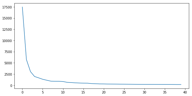
So, let’s reduce from a 7122 dimensional space to a 40 dimensional space. Now the vector associated to the word ‘dead’ (the 16th word) is:
emb = U[:,:40]
emb[15, :] # the 16th word `dead`
What does it mean? We can think it as relevant features from the model. Let’s sort now in this space. We can examine the closeness of, measure by cosine distance, any two words in the book. For example, I want to see how close between the word ‘dead’ and the word ‘wedding’
cos_dis(emb[15,:], emb[list_of_words.index('wedding'),:])
Print out the all words in a long list.
sorted(list_of_words, key = lambda word: cos_dis(emb[15,:],emb[list_of_words.index(word),:]))
You should get the following words in the top of the list:
['dead', 'fantastic', 'gilded', 'charles', 'covered'].
Seems be better, isn’t it?
What’s next?
This is just a very basic example demonstrating how to measure words closeness. In practice, the state-of-art method we usually turn to is the so called Word2Vec originally developed by a bunch of scientists in Google. In the next blog post, I will show how to use Word2Vec and the pretrained models from GloVe.