German Tank Problem Explained

June 13, 2020 | 6 Minute Read

Recently I came across a podcast talking about an anecdote about statisticians estimating the German monthly tank production numbers during World War II which I found it super interesting. The number of tanks production has been a classified information during World War II as it may reveal the real military strength (of course no one cares about the number of tanks now); thus it motivated the statisticians to estimate the true German tank production numbers based on the number of seized tanks by the allied forces.

Problem

Every captured tank has a serial number on it and if we assume the rigorous German have manufactured a series of tanks marked with consecutive whole numbers, beginning with serial number 1. Additionally it’s also presumed that the distribution over serial numbers becoming revealed is uniform. Let’s say we randomly sampled \(k\) numbers without replacement where the maximum serial number is \(m\). We are interested in the population maximum number \(N\). For example, we captured the tanks with the following serial numbers: (10, 9, 25) so the \(k = 3\) and \(m = 25\)

Frequentist point of view

The sample maximum \(M\) distribution can be described as \[ P_M(m) = \frac{\binom {m-1} {k-1} }{\binom N k} \] Thus the expectation of \(M\) is \[ E_M(m) = \mu_M= \sum_{m=k}^{N} m*\frac{\binom {m-1} {k-1} }{\binom N k} = \frac{k(N+1)}{k+1} \] Thus \[ N = \mu_M(1+k^{-1})-1 \] indicating we just need to estimate \(\mu_M\) and we are done! Since we have done the experiment just once (and only can be done once) thus \(\mu_M = m\). Therefore: \[ \hat{N} = m(1+k^{-1})-1 = m + \frac{m-k}{k} \]

Interpretation of the formula above

The population maximum equals to the sample maximum plus the average distance between each observed numbers. The interpretation is pretty intuitive, given the uniformity the best guess of the distance between population maximum and sample maximum is the average distance between sampled numbers.

Bayesian point of view

Frequentist is good but boring, and sometime lack important perspectives on uncertainty. I found the Bayesian point of view might be a better solution to this problem. If we have observed a number \(a\), what can it tell me about \(N\)? Furthermore, if additional numbers are revealed, how do we sequentially update our estimation of \(N\)? From Bayesian point of view, the model parameters are never fixed (same as people’s perspectives towards uncertainties), along with more data is being collected.

Likelihood function

Given the uniform distribution assumption, \(p(X=a|N) = \frac{1}{n} \mathbb I( 0< a \leq n)\) where \(\mathbb I() \) is the indicator function, taking the value 1 if the condition meets otherwise 0.

Prior distribution

It’s crucial to define a prior distribution in Bayesian analysis. So what’s the suitable form of prior in this case? We normally choose the conjugate prior to massively simplify the computations. The conjugate prior of an uniform distribution is Pareto distribution which is widely used to describe the “long tail” or “power law”.

\[ p(n) = Pareto(N; m, K)=\frac{Km^K}{N^{K+1}}\mathbb I(N \geq m). \]

It can be observed that the distribution cuts off at the threshold \(m\). And its probability decays following \(N^{-(K+1)}\)

Posterior distribution

According to the famous Bayesian formula, \[ p(N|X=a)=\frac{p(X=a|N)p(N)}{p(X=a)} \] so we can derive the poster distribution as follows (skipping the proof here)

\[ p(N|X=a) = \begin{cases} \frac{(K+1)m^{K+1}}{N^{K+2}}\mathbb I(N \geq m), \ \text{if} \ a \leq m; \\ \frac{(K+1)a^{K+1}}{N^{K+2}}\mathbb I(N \geq a), \ \text{if} \ a > m. \end{cases} \]

What does it mean?

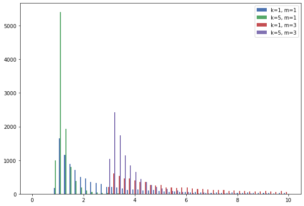
If the observed number \(a\) is less than the current sample maximum \(m\) then there is no update regarding the current known maximum however it would increase the our brief on the guess of “well the population maximum is actually \(m\)”. On the other hand, if we have observed a new number which is larger than the current sample maximum thus we need to update the possible maximum guess (at least no less than \(a\)) in the sense that we shift the histogram to the right up to the value of \(a\).

Experiments

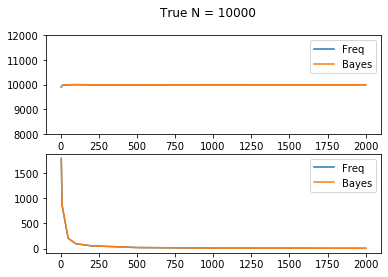
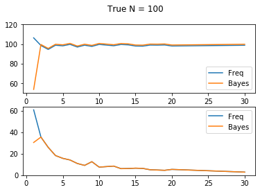
I’m pretty sure there is an engineer inside of me. So I decided to run some simulations to test which one works better.

Conclusion

It seems like there is no significant difference between Bayesian and Frequentist methods empirically, both in large true \(N = 10000\) and small true \(N = 100\) cases.

# -*- coding: utf-8 -*-
import numpy as np
from scipy.stats import randint

class GermanTanks(object):

    def __init__(self, true_N, k, T):
        self.N = true_N # the true largest number
        self.k = k # observed k numbers
        self.T = T # simulation times

    @classmethod    
    def pareto_exp(cls, k,m):
        assert k > 1
        return (k*m)/(k-1)

    @classmethod
    def bayes_mean(cls, observed):
        for i, a in enumerate(observed):
            if i == 0:
                res = a
                m = a
            else:
                m = max(observed[:i+1])
                if a <= m:
                    res = cls.pareto_exp(i+2, m)
                else:
                    res = cls.pareto_exp(i+2, a)

    @classmethod
    def freq_mean(cls, observed):
        m = max(observed)
        return m*(1+1/len(observed)) -1

    def compute_error(self):
        """
        Return the Frequentist and Bayesian means and std errors
        """

        f_mean = np.array([])
        b_mean = np.array([])

        for t in range(self.T):
            captured_tanks = randint.rvs(1, self.N, size=self.k)
            f_mean = np.append(f_mean, self.freq_mean(captured_tanks))
            b_mean = np.append(b_mean, self.bayes_mean(captured_tanks))

        return np.array([f_mean.mean(), b_mean.mean(), np.std(f_mean), np.std(b_mean)])