Summary of Survival Analysis
There is no better topic than survival in 2020. It has been 6 years since last time I sat at Prof. Richard Cook’s STAT 935: The Analysis of Survival Data class at UWaterloo, struggling with the maximum likelihood function in CoxPH model. Thanks to a recent project at work, I finally got an opportunity refreshing my memories.
Survival analysis, not getting as much attention as deep learning these days, is arguably one of the most important statistical techniques in the pharmaceutical industry. Survival analysis is used to analyze data where the time to event is of interest. The most common application is to estimate the 5-year-survival rate which is a type of survival rate for estimating the prognosis of a particular disease. Traditionally it was also used to measure lifespans of individuals despite it actually can be applied to any duration-related problems. For example, what’s the expected duration between the user subscribing to a service and then left. Another example is how long does the relationship last: a birth is then people to start to date, and a death is when they break up or divorce.
Censorship
In survival analysis, all durations are relative, i.e. all samples don’t have to start at the same starting point but are bought to a common starting point where \(t = 0\) and all samples have the survival probability equal to one when \(t = 0\). Incompletely observed responses are censored. For example, not everyone of the population will churn during the study period. However, the censored outcome does not equal to “not churn” infinitely. Removing them completely would bias the results. Additionally, to estimating the average lifetime by simply averaging everyone’s tenure as of the time of observation would severely underestimate the average user tenure. Such censorship is called right-censoring; correspondingly we may observe left-censoring or interval-censoring outcome in the data as well.
Survival models
Let \(T\) be a random lifetime taken from the population under study. The survival function \(S(t)\) of a population is defined as
\[
S(t) = Pr(T > t)
\]
i.e. the probability of surviving pass time \(t\)
Hazard function
Let’s define the hazard function \(h(t)\) at time \(t\) as
\[
h(t) = \lim_{\Delta t \rightarrow 0 } \; \frac{Pr( t \le T \le t + \Delta t | T > t)}{\Delta t}
\]
The nominator is the probability of the death event occurring at time \(t\) given that the death event has not occurred until time \(t\).
It also implies
\[
h(t) = \frac{-S'(t)}{S(t)}
\]
i.e.
\[
S(t) = \exp\left( -\int_0^t h(z) \mathrm{d}z \right)
S(t) = \exp\left(-H(t) \right)
\]
where \(H(t)\) is the cumulative hazard function.
Kaplan-Meier (K-M) estimate
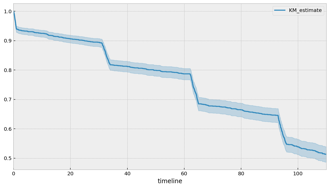
The Kaplan-Meier survival curve is defined as the probability of surviving in a given length of time while considering time in many small intervals. As a non-parametric method, Kaplan-Meier survival curve is often plotted as a first step to understand the population under study. There are three assumptions used in this analysis.
- We assume that at any time patients who are censored have the same survival prospects as those who continue to be followed.
- We assume that the survival probabilities are the same for subjects recruited early and late in the study.
- We assume that the event happens at the time specified.
The survival probability at any particular time \(t\) is calculated as follows:
\[
\hat{S_t} =\prod_{t_i \le t} \left[ 1- \frac{d_i}{n_i} \right]
\]
where \(t_i\) is a duration of study at point \(i\), \(d_i\) is number of deaths up to point \(i\) and \(n_i\) is number of individuals at risk just prior to \(t_i\). Subjects who have died, dropped out, or move out are not counted as “at risk”.
\(S\) is based upon the probability that an individual survives at the end of a time interval, on the condition that the individual was present at the start of the time interval. \(S\) is the product of these conditional probabilities. For example, the probability of a patient surviving two days after can be considered to be probability of surviving the one day multiplied by the probability surviving the second day given that patient survived the first day.

Log-rank test
Let’s talk about statistical significance, p-values and confidence intervals as they are statisticians’ favorite topics :)
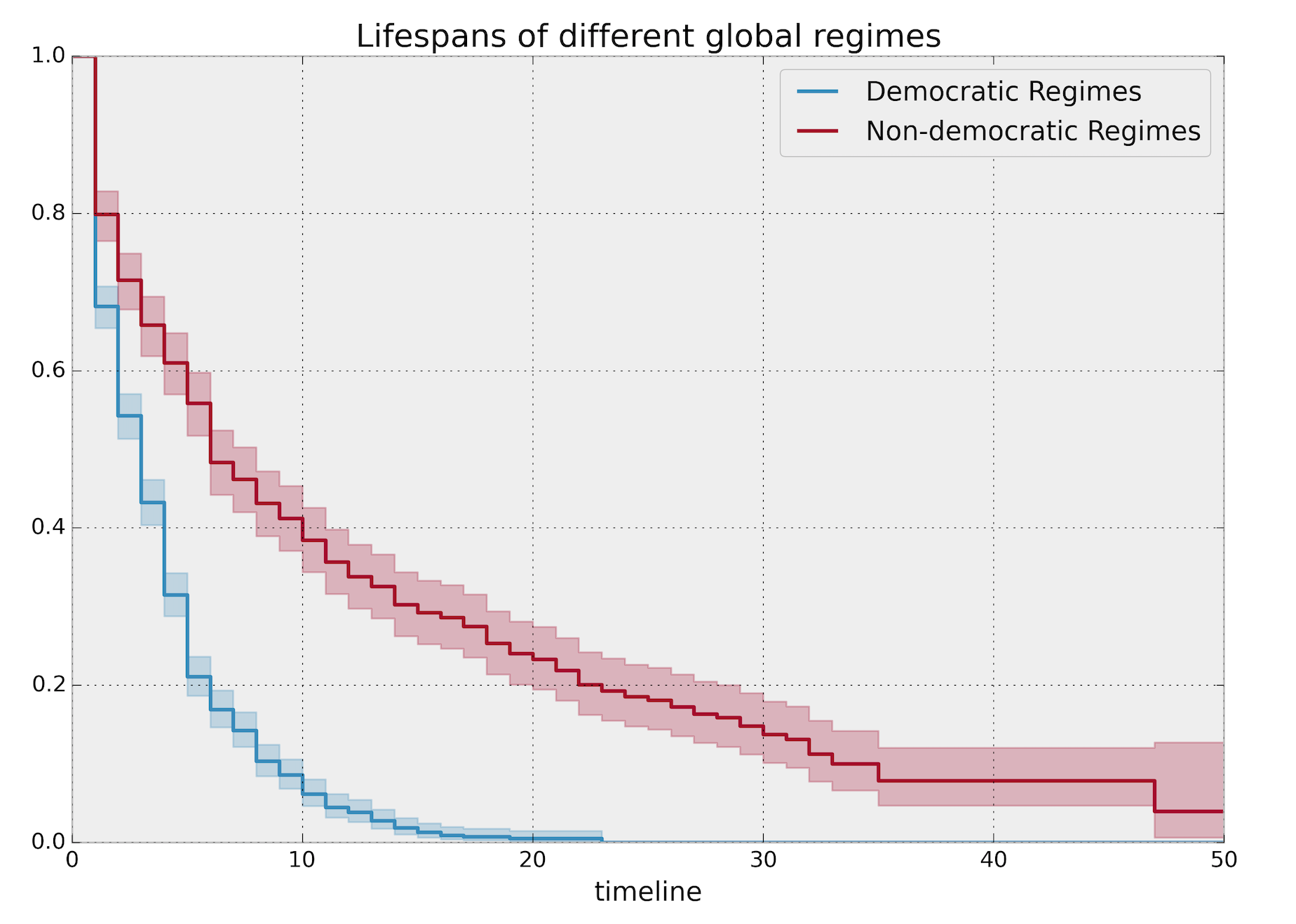
We can compare K-M curves for two different groups of subjects and establish a statistical test on two groups’ hazard functions.
\[
H_0: h_1(t) = h_2(t)
\]
Dropping the time index for the sake of simplicity, in log-rank test we calculate the expected number of events in each group i.e. \(E_1\) and \(E_2\) while \(O_1\) and \(O_2\) are the total number of observed events in each group. Note that \(O_1\) and \(O_2\) follows the hypergeometric distribution
\(\text{log-rank statistic} = \frac{O_1-E_1}{E_1} + \frac{O_2-E_2}{E_2}\).
Under the null hypothesis and large sample size, the above statistic follows the standard normal distribution by the central limit theorem (CLT).

Nelson Aalen estimator
Nelson Aalen estimator is an non-parametric estimator of the cumulative hazard function:
\[
\hat{H}(t) = \sum_{t_i \le t} \frac{d_i}{n_i}
\]
Why do we care about it? Because the sum of estimates is much more stable than the point-wise estimates.
Weibull model
Another univariate method, but parametric, to estimate the cumulative hazard function. It assumes:
\[
S(t) = \exp\left(-\left(\frac{t}{\lambda}\right)^\rho\right), \lambda >0, \rho > 0
\]
Therefore
\[
H(t) = \left(\frac{t}{\lambda}\right)^\rho
\]
Similarly, we can also consider Exponential model or Gamma model.
CoxPH model
Cox proportional hazards regression is a model to estimate the hazard rate \(h(t|x)\) by a function of \(t\) and some covariates \(x\) (i.e. features in machine learning terminology). Since its introduction in 1972, it has been the default method for survival analysis in randomized trials.
\[
\underbrace{h(t | x)}_{\text{hazard}} = \overbrace{b_0(t)}^{\text{baseline hazard}} \underbrace{\exp \overbrace{\left(\sum_{i=1}^n b_i (x_i - \overline{x_i})\right)}^{\text{log-partial hazard}}}_ {\text{partial hazard}}
\]
Assumptions
Notice that there is no time index inside the partial hazard. A fundamental assumption behind the CoxPH model is that hazards can change over time, but their ratio between levels remains a constant and the effects of the predictors are additive in one scale, i.e. the hazard functions for any two subjects at any point in time are proportional.
How to check the proportional hazard assumption
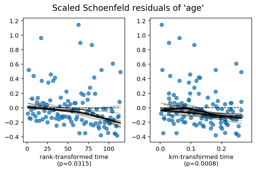
First question worth asking: do you really care about the PH assumption? Often you probably don’t because your goal is to maximize some score and you don’t care how the predictions get generated. Nevertheless, a good starting point is to rely on some graphical tool such as scaled Schoenfeld residuals against time plot. Ideally the line is flat indicating the PH assumption meets.

How to interpret the coefficients?
Recall the \(exp(\text{coeff})\) is the ratio of hazard associated with one unit change of covariate.
Concordance index
The concordance index (c-index) is a generalization of the ROC AUC to survival data, including censoring. Values of C near 0.5 indicate that the predictive score is no better than tossing a coin in determining which subject will live longer.
Stratification
If we believe the baseline hazards are very different across all subjects, the better model would have a unique baseline hazard per subgroup \(G\)
\[
h_{i |i\in G}(t) = a_i h_G(t)
\]
How about continuous variable?
We can bin and stratify it. However, there is a trade off between estimation information loss. If the bin is large, we may lose information but computing less baseline hazards. If the bin is small, we may estimate many baseline hazards.
Incorporating non-linear terms
Worth considering adding quadratic, cubic terms or splines to account for the non-linearity.
Incorporating time-varying features
To investigate the impact of the time-varying feature (such as age), we can adjust the Cox model by:
\[
h(t | x) = \overbrace{b_0(t)}^{\text{baseline}}\underbrace{\exp \overbrace{\left(\sum_{i=1}^n \beta_i (x_i(t) - \overline{x_i}) \right)}^{\text{log-partial hazard}}}_ {\text{partial hazard}}
\]
Note adding the time-varying coefficient implies a violation of the proportional hazard assumption in the sense that a covariate’s influence relative to the baseline changes over time.
Other advanced methods
- Conditional survival forest model
- Extremely randomized survival trees model
- Linear survival SVM model
- Kernel survival SVM model
What’s next
Thinking it may be enough about the theory for now. In the followup posts, I will show how to apply the survival analysis on two very interesting use cases:
- Predicting SaaS churn: not only we are able to estimate in short-term how likely the customer churn also when the event happen
- Estimating customer lifetime value: let’s focus on long-term business metric which is the customer lifetime value.
Stay tuned!